Crafting dynamic model of the control plant

Here, the dynamic model of the membrane compressor is explained.

Learn more about dynamic models

The dynamic models of physical objects are so called ‘structural diagrams’ or ‘signal graphs’. Usually, they are being constructed from the end to the beginning, i.e. from right to left.

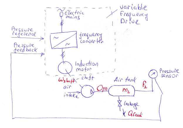
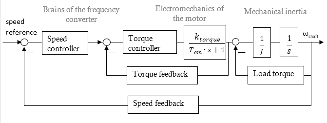
Why do we need this?

Diagrams are engineer’s best friends. It is physically impossible for humans to analyze complex interconnected systems using only textual description.

Besides, the aim of our work is to understand the structure of the control plant and properly tune the PID controller for it. To do that, it is necessary to define at least the order and character of the control plant.

The functional diagram

The figure below is called a ‘Functional diagram’.

The functional diagram is a mixture of everything: it can contain symbols of mechanical elements, electric wires, signals like reference and feedback. When designing or analyzing any system, using functional diagrams is usually the first and easiest way to understand the structure of the system.

The following table describes the variables.

Variable	Unit	Description
\(P_2\)	Pa	Pressure in the tank. The output variable
\(m_2\)	kg	Mass of the air in the tank
\(Q_{in}\)	kg/sec	Air intake mass flow rate
\(Q_{leak}\)	kg/sec	Air leakage mass flow rate
\(ω_{shaft}\)	rad/sec	Rotational speed of the shaft (motor and compressor common speed)

The structural model of compressor and the air tank

The relation between the pressure in the tank is described by the equation of the ideal gas

\[P_2 \cdot V_2 = \frac{m_2}{M_{air}}\cdot R \cdot T_2\]

where  P₂ is the pressure in the tank,

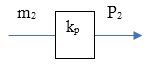
        V₂ is its volume;

        m₂ is the mass of the air in the tank;

        M₂ is the molar mass of the air;

        R=8.314 is the molar gas constant (also known as the gas constant, universal gas constant, or ideal gas constant);

        T2 is the absolute temperature [K] of the air in the tank.

The equation is given only to illustrate the dependency of pressure and mass. None of these variable except P₂ we shall use in calculations, thus we don’t need their values.

Considering that all other variables in this equation are constant, we can assume that the pressure is proportional to the mass of the air:

\[P_2 = k_p \cdot m-2\]

where k_p is a pressure coefficient.

Thus, this element is represented by a simple gain

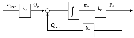
The mass m₂ of the air currently present in the reservoir is an integral of the mass flow. The latter is the difference between the intake Q_in and leakage Q_leak mass flow rates:

\[m_2 = \int{(Q_{in}-Q_{leak})\cdot dt}\]

We assume that the leakage is proportional to the pressure in the tank, the bigger the pressure – the fast the air leaks out

\[Q_{leak} = k_L \cdot P_2\]

Finally, the air intake Q_in depends on the number of reciprocating cycles per minute. The more frequent membrane ‘exhales’ are, the more air supplies the compressor. In other words, we simply assume that Q_in is proportional to the motor rotation speed

\[ Q_{in}=k_{\omega}\cdot \omega\]

The structural diagram is shown in the figure below.

Integration in Laplace transform is represented as \(\frac{1}{2}\). Hereinafter we are use this designation.

Thus, the total transfer function of this part of the control plant will be

\[W(s)=\frac{P_2}{\omega_{shaft}}=\frac{k_\omega}{T_{compressor} \cdot s + 1}\]

where \(T_{compressor}=\frac{1}{k_P \cdot k_L}\) – relatively big compressor’s time constant.

It is so-called aperiodic, or inertial element.

Note that the control plant is not only compressor, but all the part of the system between PID-controller and pressure sensor.

Learn more:

Model of the variable frequency drive

Considering that the process of pressure regulation is very slow, we can represent the electric drive (which is frequency converter with its control system and electric motor) as two folded loops: the torque loop and the speed loop:

The torque controller ‘compensates’ the electromagnetic time constant T_em. The VFD develops the torque very quickly, the time delay may even be neglected.

However, there is still mechanical inertia J. It takes time for the motor to speed up.

Besides, all VFDs have so-called ‘Ramp time’ setting – a non-zero time when speed reference achieves the given value.

Thus, a VFD is also a non-linear first-order aperiodic element.

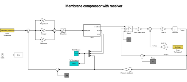
The full model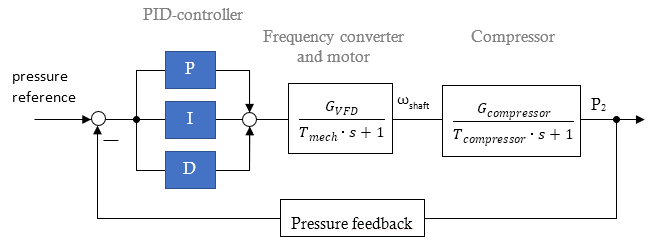

Assumptions

Understanding assumptions is more important than it might seem. Often it means the difference between whether or not the equipment will work.

Any model is idealistic. Models never represent all the physical phenomena in the control plants.

Our model has the following assumptions and deviations of the idealistic case

• The compressor is actually an asymmetrical control plant. It is able to generate only positive intake and thus increase the pressure. It cannot ‘suck off’ the air from the air reservoir to decrease it. The pressure can only reduce itself due to the leaks.
• The air temperature in the chambers and reservoir is assumed constant while it is not.
• It is assumed that the air intake is proportional to the shaft rotation speed and doesn’t depend on the actual pressure in the reservoir. Actually, it is somehow non-linearly depend on the difference of pressures in the compressor chambers and the air tank. The higher the pressure in the tank, the less is the inflow.
• Thus, the actual control plant is non-linear.

Learn more: Implementation in Matlab

The diagram below illustrates the implementation of the dynamic model in MatLAB^®Simulink.

Subsystem of VFD will look like

The figure below illustrates the transients in the system