PID-control

Control quality

Controllers and feedbacks are attached to systems in order to improve the quality of process control, or simply, the control quality.

Before starting to improve something, it is important to ask yourself “What are we trying to improve?”.

The following table classifies the control quality criteria.

Static	Dynamic
Accuracy/precision vs. static error Smoothness Control range	Overshot How fast Oscillations Dynamic error

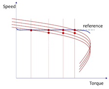
The static performances are pretty obvious: we need minimal mismatch between the given and actual values, thus minimal error. The system is not smooth when the control principle allows only discrete setting of e.g. drive speed. The control range refers to the ratio of minimal and maximal values that system is able to achieve.

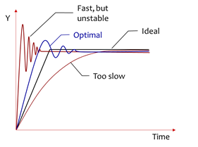
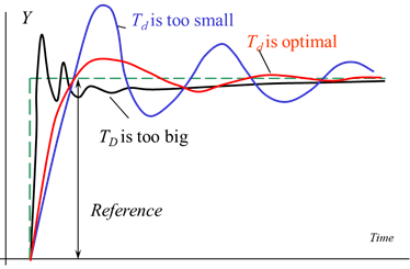
The diagrams illustrating dynamic criteria have time as X-axis. So, dynamics is about how fast the system can get into the desired state and how exactly the process evolves in time. They also describe the shape of the transient curve.

An engineer can estimate the quality at a glance, telling how ‘good’ or ‘bad’ the system is tuned. But preferably, there should be a certain measure of quality, or quantitative indices. Those are illustrated in the diagram below.

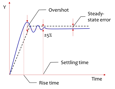
The Y-coordinate is typically speed, position, temperature, pressure etc.

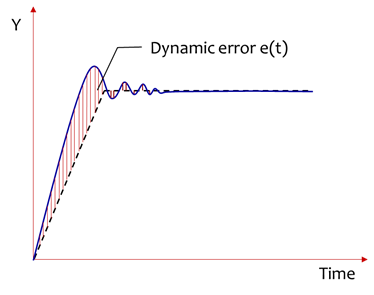
Learn more: dynamic error

\[IAE = \int^{\infty}_0{\lvert {e(t)} \rvert dt}\]	Integral of absolute error
\[ISE = \int^{\infty}_0{ [{e(t)} ]^2 dt}\]	Integral of squared error
\[ITAE = \int^{\infty}_0{t \lvert {e(t)} \rvert dt}\]	Integral of time multiplied by absolute error
\[ITSE = \int^{\infty}_0{t [{e(t)} ]^2 dt}\]	Integral of time multiplied by squared error

PID components and transients

In general, controllers of dynamic systems contain three components:

• proportional (P),
• integral (I), and
• derivative (D).

Thus, PID-controller.

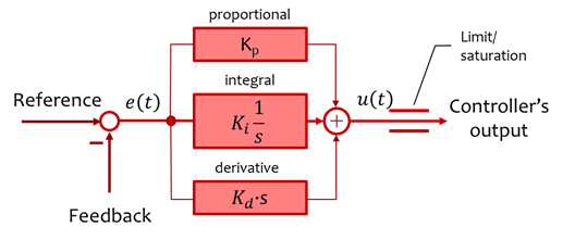
The mathematical expression of the controller’s output is

\[u(t)=K_p e(t) + K_i \int^t_0{e(t) dt} + K_d \frac{de(t)}{dt}\]

where \(e(t)\) is the error value, the difference between the desired setpoint and the feedback (actual process value).

Consider that in real applications the output is always limited to a certain value.

By tuning the three coefficients K_p, K_i and K_d it is possible to improve the control quality.

Learn more: the PID controller theory

It is necessary to understand the behavior of the system, its reaction to each of the three P-, I- and D- terms.

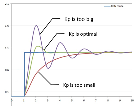
Proportional gain

Idea	Just take the input error signal \(e(t)\) and multiply it by Kp
Effect	The proportional term reduces the rise time (makes the system more fast) and reduces the steady-state error Increasing Kp makes the system more unstable
Specifics	It can only work if the error \(e(t)\) is non-zero

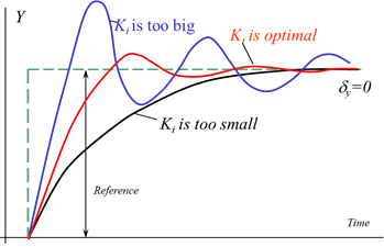
Integral gain

Idea	This component accounts for the past values of the input signal and integrates them
Effect	The purpose if the integral component is to eliminate the steady-state error Increasing Ki makes the system more unstable
Specifics	Can work even if \(e(t)=0\)

Learn more: why systems with integral component are called ‘Astatic’?

‘Astatic’ means there is no steady-state (‘static’) error. It is because an integral of a function is

\[\int{e(t)dt}=E(t)+C\]

Even if \(e(t)=0\)

\[\int{0 \cdot dt} = C\]

I.e. the integral component of the regulator will keep producing the output signal even if the error on its input is zero.

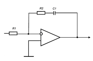
In analog control systems with differential amplifiers it is the capacitor that holds the charge and thus providing the output voltage even if the input signal is zero

Derivative gain

Idea	The derivative (or differential) component tries to predict the future values of \(e(t)\) basing on its rate of change and acts according to it
Effect	The purpose if the derivative component is improve system’s stability Increasing Kd up to certain values damps the oscillations and ‘soothes’ the system
Specifics	Certain too hich values of Kd make the system unstable This component amplifies the noise and thus makes the system vulnerable

Summary on P-, I-, D-

Parameter	Increasing the P-, I-, D- parameter results in
	Rise time	Overshoot	Settling time	Steady-state error	Stability
Kp	Decrease	Increase	Small change	Decrease	Degrade
Ki	Decrease	Increase	Increase	Eliminate	Degrade
Kd	Minor change	Decrease	Decrease	No effect in theory	Improve if Kd is mall

The animation below (taken from here) illustrates how the P-, I- and D- components change the step-response

Learn more: Quantitative methods of PID-controller parametrization

The above given recommendations help you understanding the behavior of the system. You can anticipate the response of your system onto the change of controller’s gains. In 99% of cases in the real life, engineers tune their systems manually.

However, tthe control engineering theory has lots of approaches for the a priori (which means ‘before experiment’) calculation of the optimal PID gains.

The following table summarizes the most common methods.

Method	Advantages	Disadvantages
Manual tuning	Doesn’t require the knowledge of the control plant’s parameters	You can damage the machinery by exceeding the permissible output values
Ziegler–Nichols [b]	Semi-experiment method. Simple and robust	Aggressive tuning, you can damage the machinery by exceeding the permissible output values
Tyreus Luyben	Proven method	Aggressive tuning, you can damage the machinery by exceeding the permissible output values
Cohen–Coon	Good process models.	Some mathematics; only good for first-order processes
Åström-Hägglund	Can be used for auto tuning; amplitude is minimum so this method has lowest process upset	The process itself is inherently oscillatory